Python-Numpy简单了解

Alt Text

Numpy 高效的运算工具
Numpy的优势
ndarray属性
基本操作
- ndarray.方法()
- numpy.函数名()
ndarray运算
- 逻辑运算
- 统计运算
- 数组间运算
合并、分割、IO操作、数据处理

1. Numpy优势

1.1 Numpy介绍 - 数值计算库

num - numerical 数值化的
py - python
ndarray
- n - 任意个
- d - dimension 维度
- array - 数组

1.2 ndarray介绍

python

import numpy as np

score = np.array([[80, 89, 86, 67, 79],
                  [78, 97, 89, 67, 81],
                  [90, 94, 78, 67, 74],
                  [91, 91, 90, 67, 69],
                  [76, 87, 75, 67, 86],
                  [70, 79, 84, 67, 84],
                  [94, 92, 93, 67, 64],
                  [86, 85, 83, 67, 80]])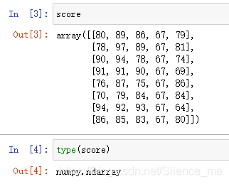

Alt Text

1.3 ndarray与Python原生list运算效率对比

python

import random
import time

# 生成一个大数组
python_list = []

for i in range(100000000):
  python_list.append(random.random())
ndarray_list = np.array(python_list)

# 原生pythonlist求和
t1 = time.time()
a = sum(python_list)
t2 = time.time()
d1 = t2 - t1

# ndarray求和
t3 = time.time()
b = np.sum(ndarray_list)
t4 = time.time()
d2 = t4 - t3

d1= 0.7309620380401611 d2= 0.12980318069458008

1.4 ndarray的优势

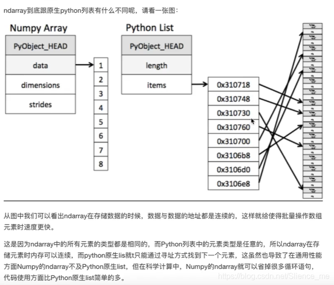
存储风格 ndarray - 相同类型 - 通用性不强 list - 不同类型 - 通用性很强
并行化运算 ndarray支持向量化运算
底层语言 C语言，解除了GIL

2. 认识N维数组-ndarray属性

2.1 ndarray的属性

shape
- ndim ：看看维度
- size ：看看大小
dtype
- itemsize ：一个元素所占大小
在创建ndarray的时候，如果没有指定类型
默认
- 整数 int64
- 浮点数 float64

python

array([[80, 89, 86, 67, 79],
       [78, 97, 89, 67, 81],
       [90, 94, 78, 67, 74],
       [91, 91, 90, 67, 69],
       [76, 87, 75, 67, 86],
       [70, 79, 84, 67, 84],
       [94, 92, 93, 67, 64],
       [86, 85, 83, 67, 80]])

score.shape  # (8, 5)
score.ndim  # 2
score.size  # 40
score.dtype  # dtype('int64')
score.itemsize  # 8

2.2 ndarray的形状

python

a = np.array([[1, 2, 3], [4, 5, 6]])
b = np.array([1, 2, 3, 4])
c = np.array([[[1, 2, 3], [4, 5, 6]], [[1, 2, 3], [4, 5, 6]]])

a  # array([[1, 2, 3],
b  # array([1, 2, 3, 4])
c  # array([[[1, 2, 3],[4, 5, 6]],[[1, 2, 3],[4, 5, 6]]])
a.shape  # (2, 3)
b.shape  # (4,)
c.shape  # (2, 2, 3)

2.3 ndarray的类型

python

type(score.dtype)
< type
'numpy.dtype' >

# 指定类型
# 创建数组的时候指定类型
np.array([1.1, 2.2, 3.3], dtype="float32")

dtype是numpy是numpy.dtype类型，先看看对数组来说都有哪些类型

名称	描述	简写
np.bool	用一个字节存储的布尔类型(True或False)	'b'
np.int8	一个字节大小，-128~127	'i'
np.int16	整数，-32768至32767	'i2'
np.int32	整数，-231至232 -1	'i4'
np.int64	整数，-263至263 -1	'i8'
np.uint8	无符号整数，0~255	'u'
np.uint16	无符号整数，0~65535	'u2'
np.uint32	无符号整数，0~2 ** 32 -1	'u4'
np.uint64	无符号整数，0~2 ** 64 -1	'u8'
np.float16	半精度浮点数：16位，正负号1位，指数5位，精度10位	'f2'
np.float32	单精度浮点数：32位，正负号1位，指数8位，精度23位	'f4'
np.float64	双度浮点数：64位，正负号1位，指数11位，精度52位	'f8'
np.complex64	复数，分别用两个32位浮点数表示实部和虚部	'c8'
np.complex128	复数，分别用两个64位浮点数表示实部和虚部	'c16'
np.object_	python对象	'O'
np.string	字符串	'S'
np.unicode	unicode类型	'U'

3. 基本操作

adarray.方法()
np.函数名()
- np.array()

3.1 生成数组的方法

3.1.1 生成0和1

np.zeros(shape)
np.ones(shape)

python

# 1 生成0和1的数组
np.zeros(shape=(3, 4), dtype="float32")
-----------------------------------------
array([[0., 0., 0., 0.],
       [0., 0., 0., 0.],
       [0., 0., 0., 0.]], dtype=float32)

python

np.ones(shape=[2, 3], dtype=np.int32)
-----------------------------------------
array([[1, 1, 1],
       [1, 1, 1]], dtype=int32)

3.1.2 从现有数组中生成

np.array() np.copy() 深拷贝
np.asarray() 浅拷贝

python

data1 = np.array(score)
data2 = np.asarray(score)
data3 = np.copy(score)
score[3, 1] = 10000

修改source，data2改变，data1，data3不改变

3.1.3 生成固定范围的数组

np.linspace(0, 10, 100)
- [0, 10] 等距离生成个数
np.arange(a, b, c)
- range(a, b, c)
  - [a, b) c是步长

python

np.linspace(0, 10, 5)
# array([ 0. ,  2.5,  5. ,  7.5, 10. ])
np.arange(0, 11, 5)
# array([ 0,  5, 10])

3.1.4 生成随机数组

分布状况 - 直方图

均匀分布每组的可能性相等
正态分布 σ 幅度、波动程度、集中程度、稳定性、离散程度

均匀分布uniform
- low：float类型，此概率的均值(对应着整个分布的中心centre)
- scale：float类型，此概率分布的标准差(对应于分布的宽度，scale越大越矮胖，越小越瘦高)
- size：int or tuple of ints 输出的shape，默认位None，只输出一个值

python

import matplotlib.pyplot as plt
import numpy as np

data1 = np.random.uniform(low=-1, high=1, size=1000000)
array([-0.49795073, -0.28524454, 0.56473937, ..., 0.6141957,
       0.4149972, 0.89473129])
# 1、创建画布
plt.figure(figsize=(20, 8), dpi=80)

# 2、绘制直方图
plt.hist(data1, 1000)

# 3、显示图像
plt.show()

Alt Text

正态分布normal
- low：此概率的均值(对应着整个分布的中心centre)
- scale：float此概率分布的标准差(对应于分布的宽度，scale越大越矮胖，越小越瘦高)
- size：int or tuple of ints 输出的shape，默认位None，只输出一个值

python

# 正态分布
data2 = np.random.normal(loc=1.75, scale=0.1, size=1000000)
# 1、创建画布
plt.figure(figsize=(20, 8), dpi=80)

# 2、绘制直方图
plt.hist(data2, 1000)

# 3、显示图像
plt.show()

Alt Text

3.2 数组的索引、切片

python

stock_change = np.random.normal(loc=0, scale=1, size=(8, 10))
# 返回结果
array([[-0.03469926, 1.68760014, 0.05915316, 2.4473136, -0.61776756, -0.56253866, -1.24738637, 0.48320978, 1.01227938,
        -1.44509723],
       [-1.8391253, -1.10142576, 0.09582268, 1.01589092, -1.20262068, 0.76134643, -0.76782097, -1.11192773, 0.81609586,
        0.07659056],
       [-0.74293074, -0.7836588, 1.32639574, -0.52735663, 1.4167841, 2.10286726, -0.21687665, -0.33073563, -0.46648617,
        0.07926839],
       [0.45914676, -0.78330377, -1.10763289, 0.10612596, -0.63375855, -1.88121415, 0.6523779, -1.27459184, -0.1828502,
        -0.76587891],
       [-0.50413407, -1.35848099, -2.21633535, -1.39300681, 0.13159471, 0.65429138, 0.32207255, 1.41792558, 1.12357799,
        -0.68599018],
       [0.3627785, 1.00279706, -0.68137875, -2.14800075, -2.82895231, -1.69360338, 1.43816168, -2.02116677, 1.30746801,
        1.41979011],
       [-2.93762047, 0.22199761, 0.98788788, 0.37899235, 0.28281886, -1.75837237, -0.09262863, -0.92354076, 1.11467277,
        0.76034531],
       [-0.39473551, 0.28402164, -0.15729195, -0.59342945, -1.0311294, -1.07651428, 0.18618331, 1.5780439, 1.31285558,
        0.10777784]])

# 获取第一个股票的前3个交易日的涨跌幅数据
stock_change[0, :3]
# 返回结果
array([-0.03469926, 1.68760014, 0.05915316])

一维、二维、三维的数组如何索引？

python

# 三维，一维
a1 = np.array([[[1, 2, 3], [4, 5, 6]], [[12, 3, 34], [5, 6, 7]]])
# 返回结果
array([[[1, 2, 3],
        [4, 5, 6]],

       [[12, 3, 34],
        [5, 6, 7]]])
# 索引、切片
a1.shape  # (2, 2, 3)
a1[1, 0, 2]  # 34

# 修改
a1[1, 0, 2] = 100000
# 返回结果
array([[[1, 2, 3],
        [4, 5, 6]],

       [[12, 3, 100000],
        [5, 6, 7]]])

3.3 形状修改

ndarray.reshape(shape) 返回新的ndarray，原始数据没有改变
ndarray.resize(shape) 没有返回值，对原始的ndarray进行了修改
ndarray.T 转置行变成列，列变成行

ndarray.reshape(shape)返回新的ndarray，原始数据没有改变

python

# 需求：让刚才的股票行、日期列反过来，变成日期行，股票列
stock_change
# 返回结果
array(
  [[-0.03469926, 1.68760014, 0.05915316, 2.4473136, -0.61776756,
    -0.56253866, -1.24738637, 0.48320978, 1.01227938, -1.44509723],
   [-1.8391253, -1.10142576, 0.09582268, 1.01589092, -1.20262068,
    0.76134643, -0.76782097, -1.11192773, 0.81609586, 0.07659056],
   [-0.74293074, -0.7836588, 1.32639574, -0.52735663, 1.4167841,
    2.10286726, -0.21687665, -0.33073563, -0.46648617, 0.07926839],
   [0.45914676, -0.78330377, -1.10763289, 0.10612596, -0.63375855,
    -1.88121415, 0.6523779, -1.27459184, -0.1828502, -0.76587891],
   [-0.50413407, -1.35848099, -2.21633535, -1.39300681, 0.13159471,
    0.65429138, 0.32207255, 1.41792558, 1.12357799, -0.68599018],
   [0.3627785, 1.00279706, -0.68137875, -2.14800075, -2.82895231,
    -1.69360338, 1.43816168, -2.02116677, 1.30746801, 1.41979011],
   [-2.93762047, 0.22199761, 0.98788788, 0.37899235, 0.28281886,
    -1.75837237, -0.09262863, -0.92354076, 1.11467277, 0.76034531],
   [-0.39473551, 0.28402164, -0.15729195, -0.59342945, -1.0311294,
    -1.07651428, 0.18618331, 1.5780439, 1.31285558, 0.10777784]])

stock_change.reshape((10, 8))
# 返回结果
array(
  [[-0.03469926, 1.68760014, 0.05915316, 2.4473136, -0.61776756,
    -0.56253866, -1.24738637, 0.48320978],
   [1.01227938, -1.44509723, -1.8391253, -1.10142576, 0.09582268,
    1.01589092, -1.20262068, 0.76134643],
   [-0.76782097, -1.11192773, 0.81609586, 0.07659056, -0.74293074,
    -0.7836588, 1.32639574, -0.52735663],
   [1.4167841, 2.10286726, -0.21687665, -0.33073563, -0.46648617,
    0.07926839, 0.45914676, -0.78330377],
   [-1.10763289, 0.10612596, -0.63375855, -1.88121415, 0.6523779,
    -1.27459184, -0.1828502, -0.76587891],
   [-0.50413407, -1.35848099, -2.21633535, -1.39300681, 0.13159471,
    0.65429138, 0.32207255, 1.41792558],
   [1.12357799, -0.68599018, 0.3627785, 1.00279706, -0.68137875,
    -2.14800075, -2.82895231, -1.69360338],
   [1.43816168, -2.02116677, 1.30746801, 1.41979011, -2.93762047,
    0.22199761, 0.98788788, 0.37899235],
   [0.28281886, -1.75837237, -0.09262863, -0.92354076, 1.11467277,
    0.76034531, -0.39473551, 0.28402164],
   [-0.15729195, -0.59342945, -1.0311294, -1.07651428, 0.18618331,
    1.5780439, 1.31285558, 0.10777784]])

ndarray.resize(shape)没有返回值，对原始的ndarray进行了修改

python

stock_change.shape  # (8, 10)
stock_change.resize((10, 8))
stock_change.shape  # (10, 8)

ndarray.T转置行变成列，列变成行

python

stock_change.T

3.4 类型修改

ndarray.astype(type)
ndarray序列化到本地
ndarray.tostring()

python

stock_change.astype("int32")
# 返回结果
array([[0, 1, 0, 2, 0, 0, -1, 0, 1, -1],
       [-1, -1, 0, 1, -1, 0, 0, -1, 0, 0],
       [0, 0, 1, 0, 1, 2, 0, 0, 0, 0],
       [0, 0, -1, 0, 0, -1, 0, -1, 0, 0],
       [0, -1, -2, -1, 0, 0, 0, 1, 1, 0],
       [0, 1, 0, -2, -2, -1, 1, -2, 1, 1],
       [-2, 0, 0, 0, 0, -1, 0, 0, 1, 0],
       [0, 0, 0, 0, -1, -1, 0, 1, 1, 0]], dtype=int32)

stock_change.tobytes()
b'\x95&\x99\xdd\x19\xc4\xa1\xbfm8\x88\x00i\x00\xfb?\x92\xbc\x81\xa1RI\xae?\xa2\x95x&\x19\x94\x03@\x9f?\xbev\xc0\xc4\xe3\xbf\x87\xf4H\x13Q\x00\xe2\xbf\x9eM\x85hK\xf5\xf3\xbf\x17mZ\xb2\xe8\xec\xde?U\xca\xd4\xdbK2\xf0?G\xc6\xbbD\x1e\x1f\xf7\xbf\x9f-\xb0\xa5\x0em\xfd\xbf\x9b\xd0h\x9dp\x9f\xf1\xbfyH\x8e\xc3\xd5\x87\xb8?\x1d\x89v\xd5\x16A\xf0?\x89Aj-\xef=\xf3\xbf\xbc\x8ea/\xf3\\\xe8?\x94\xb8\xbaJ\xfd\x91\xe8\xbfv\xc0\x92\xbct\xca\xf1\xbf\x82\x82\x19\x11u\x1d\xea?\xf2.\x96Qp\x9b\xb3?g\xed\xef\xb0\x16\xc6\xe7\xbf\xf2\xbf!\x9c\xbb\x13\xe9\xbf\x7fv\x1e\xbd\xea8\xf5?\x1e \x9d\x02\x1b\xe0\xe0\xbf?\x99O\xce%\xab\xf6?\x84;\xb9\x11\xac\xd2\x00@p\xe3\xa07\x9d\xc2\xcb\xbfop\x94\xc4\xc5*\xd5\xbfN\x15)\xca\xe8\xda\xdd\xbf4\xa8\x8b\xf1\xeeJ\xb4?Qd\x8e\x1c\xa9b\xdd?\xc8\x92\xb6\x10\xd3\x10\xe9\xbf\xf1\x80\x87C\xdd\xb8\xf1\xbf\x18\x02B \x12+\xbb?Xv\xb4\x02\xc0G\xe4\xbf\xa6,\x8a\x02t\x19\xfe\xbf\xb4\xc9\xaf\x9cG\xe0\xe4?wCsj\xbad\xf4\xbf\xbc\xb1\xd5\xa9\xa2g\xc7\xbf\xbc\xc6\x8d{\x14\x82\xe8\xbf>\xf7\xae\xc6\xdd!\xe0\xbf\xacB\x9c\x90V\xbc\xf5\xbfb\xae\xfa\x06\x0e\xbb\x01\xc0_B\xe1\x82\xc1I\xf6\xbfw\x9f\xb6m\x18\xd8\xc0?\x93\xcb\x8e{\xf4\xef\xe4?\xfe\xc1\xba,\xd6\x9c\xd4?k\x85)\xbc\xd2\xaf\xf6?{g\x82\xea,\xfa\xf1?s}\xaf\xad\xa1\xf3\xe5\xbfD(cM\xc37\xd7?(\x1a\xff\xect\x0b\xf0?7e\x80\xce\xda\xcd\xe5\xbf"\xd5\xe1\x03\x1b/\x01\xc0\x94\x85?\xbf\xb1\xa1\x06\xc0w\x08\x14\xdc\xff\x18\xfb\xbf\x9f\x1eL\xd2\xb5\x02\xf7?\xb0-5{Y+\x00\xc0;\xf5<\x94c\xeb\xf4?a\x8f\xb1\xd6u\xb7\xf6?%Kr)?\x80\x07\xc0\x9e\x1c%\xedjj\xcc?F\xa0C\t\xc7\x9c\xef?\xf3\xc3\xfd\x1eiA\xd8?\xcc\x9e\x84D\xb4\x19\xd2?\xdd$J\x10K"\xfc\xbf\xe6E\xb3\x95\x82\xb6\xb7\xbf\x0cN\xa4Z\xa5\x8d\xed\xbf\x96\xdd\xee\x1c\xb3\xd5\xf1?\x05\x8c\x12\xb0\xbfT\xe8?/\xa5\x1a\xb9XC\xd9\xbf~Z!\x1ci-\xd2?\x1f\xe4\xe3\x83$"\xc4\xbf_&\xc5\xc0_\xfd\xe2\xbf\xbf\x16\xac\x8b\x81\x7f\xf0\xbf\xf7\xba)\tg9\xf1\xbf\xb7q\x8c\xd7\xda\xd4\xc7?\x98P\xb7\xf4\xaa?\xf9?\x8c\x98P\xdbt\x01\xf5?t\xd8 -T\x97\xbb?'

3.5 数组的去重

set()：只能处理一维
np.unique()

python

temp = np.array([[1, 2, 3, 4], [3, 4, 5, 6]])
# 返回结果
array([[1, 2, 3, 4],
       [3, 4, 5, 6]])
np.unique(temp)
# 返回结果
array([1, 2, 3, 4, 5, 6])

set(temp.flatten())  # 将多维降维成一维，然后用set去重 只能处理一维
# 返回结果
{1, 2, 3, 4, 5, 6}

4. ndarray运算

4.1 逻辑运算

布尔索引
通用判断函数
- np.all(布尔值)
  - 只要有一个False就返回False，只有全是True才返回True
- np.any()
  - 只要有一个True就返回True，只有全是False才返回False
np.where（三元运算符）
- np.where(布尔值, True的位置的值, False的位置的值)

python

stock_change = np.random.normal(loc=0, scale=1, size=(8, 10))
# 返回结果
array([[1.46338968, -0.45576704, 0.29667843, 0.16606916, 0.46446682, 0.83167611, -1.35770374, -0.65001192, 1.38319911,
        -0.93415832],
       [0.36775845, 0.24078108, 0.122042, 1.19314047, 1.34072589, 0.09361683, 1.19030379, 1.4371421, -0.97829363,
        -0.11962767],
       [-1.48252741, -0.69347186, 0.91122464, -0.30606473, 0.41598897, 0.79542753, -0.01447862, -1.49943117,
        -0.23285809, 0.42806777],
       [0.39438905, -1.31770556, 1.7344868, -1.52812773, -0.47703227, -0.3795497, -0.88422651, 1.37510973, -0.93622775,
        0.49257673],
       [-0.9822216, -1.09482936, -0.81834523, 0.57335311, 0.97390091, 0.05314952, -0.58316743, 0.19264426, 0.02081861,
        0.84445247],
       [0.41739964, -0.26826893, -0.70003442, -0.58593912, 0.86546709, -1.30304864, 0.05254567, -1.73976785,
        -0.43532247, 0.4760526],
       [-0.21739882, 0.52007085, -0.60160491, 0.57108639, 1.03303301, -0.69172579, 1.04716985, -0.22985706, -0.11125069,
        0.87722923],
       [-0.183266, 0.56273065, 0.29357786, -0.19343363, -1.54547303, -0.31977163, -0.00659025, 0.48160678, 0.88443604,
        -0.48456825]])
--------------------------------------------------
# 逻辑判断, 如果涨跌幅大于0.5就标记为True 否则为False
stock_change > 0.5
# 返回结果
array([[True, False, False, False, False, True, False, False, True, False],
       [False, False, False, True, True, False, True, True, False, False],
       [False, False, True, False, False, True, False, False, False, False],
       [False, False, True, False, False, False, False, True, False, False],
       [False, False, False, True, True, False, False, False, False, True],
       [False, False, False, False, True, False, False, False, False, False],
       [False, True, False, True, True, False, True, False, False, True],
       [False, True, False, False, False, False, False, False, True, False]])
--------------------------------------------------
stock_change[stock_change > 0.5] = 1.1
# 返回结果
array([[1.1, -0.45576704, 0.29667843, 0.16606916, 0.46446682, 1.1, -1.35770374, -0.65001192, 1.1, -0.93415832],
       [0.36775845, 0.24078108, 0.122042, 1.1, 1.1, 0.09361683, 1.1, 1.1, -0.97829363, -0.11962767],
       [-1.48252741, -0.69347186, 1.1, -0.30606473, 0.41598897, 1.1, -0.01447862, -1.49943117, -0.23285809, 0.42806777],
       [0.39438905, -1.31770556, 1.1, -1.52812773, -0.47703227, -0.3795497, -0.88422651, 1.1, -0.93622775, 0.49257673],
       [-0.9822216, -1.09482936, -0.81834523, 1.1, 1.1, 0.05314952, -0.58316743, 0.19264426, 0.02081861, 1.1],
       [0.41739964, -0.26826893, -0.70003442, -0.58593912, 1.1, -1.30304864, 0.05254567, -1.73976785, -0.43532247,
        0.4760526], [-0.21739882, 1.1, -0.60160491, 1.1, 1.1, -0.69172579, 1.1, -0.22985706, -0.11125069, 1.1],
       [-0.183266, 1.1, 0.29357786, -0.19343363, -1.54547303, -0.31977163, -0.00659025, 0.48160678, 1.1, -0.48456825]])

python

# 判断stock_change[0:2, 0:5]是否全是上涨的
stock_change[0:2, 0:5] > 0
# 返回结果
array([[True, False, True, True, True],
       [True, True, True, True, True]])
--------------------------------------------------
np.all(stock_change[0:2, 0:5] > 0)
# 返回结果
False
--------------------------------------------------
# 判断前5只股票这段期间是否有上涨的
np.any(stock_change[:5, :] > 0)
# 返回结果
True

python

# 判断前四个股票前四天的涨跌幅 大于0的置为1，否则为0
temp = stock_change[:4, :4]
# 返回结果
array([[1.1, -0.45576704, 0.29667843, 0.16606916],
       [0.36775845, 0.24078108, 0.122042, 1.1],
       [-1.48252741, -0.69347186, 1.1, -0.30606473],
       [0.39438905, -1.31770556, 1.1, -1.52812773]])
--------------------------------------------------
np.where(temp > 0, 1, 0)
# 返回结果
array([[1, 0, 1, 1],
       [1, 1, 1, 1],
       [0, 0, 1, 0],
       [1, 0, 1, 0]])
--------------------------------------------------
temp > 0
# 返回结果
array([[True, False, True, True],
       [True, True, True, True],
       [False, False, True, False],
       [True, False, True, False]])
--------------------------------------------------
np.where([[True, False, True, True],
          [True, True, True, True],
          [False, False, True, False],
          [True, False, True, False]], 1, 0)
# 返回结果
array([[1, 0, 1, 1],
       [1, 1, 1, 1],
       [0, 0, 1, 0],
       [1, 0, 1, 0]])
--------------------------------------------------
# 判断前四个股票前四天的涨跌幅 大于0.5并且小于1的，换为1，否则为0
# 判断前四个股票前四天的涨跌幅 大于0.5或者小于-0.5的，换为1，否则为0
# (temp > 0.5) and (temp < 1)
np.logical_and(temp > 0.5, temp < 1)
# 返回结果
array([[False, False, False, False],
       [False, False, False, False],
       [False, False, False, False],
       [False, False, False, False]])
--------------------------------------------------
np.where([[False, False, False, False],
          [False, False, False, False],
          [False, False, False, False],
          [False, False, False, False]], 1, 0)
# 返回结果
array([[0, 0, 0, 0],
       [0, 0, 0, 0],
       [0, 0, 0, 0],
       [0, 0, 0, 0]])
--------------------------------------------------
np.where(np.logical_and(temp > 0.5, temp < 1), 1, 0)
# 返回结果
array([[0, 0, 0, 0],
       [0, 0, 0, 0],
       [0, 0, 0, 0],
       [0, 0, 0, 0]])
--------------------------------------------------
np.logical_or(temp > 0.5, temp < -0.5)
# 返回结果
array([[True, False, False, False],
       [False, False, False, True],
       [True, True, True, False],
       [False, True, True, True]])
--------------------------------------------------
np.where(np.logical_or(temp > 0.5, temp < -0.5), 11, 3)
# 返回结果
array([[11, 3, 3, 3],
       [3, 3, 3, 11],
       [11, 11, 11, 3],
       [3, 11, 11, 11]])

4.2 统计运算

axis轴的取值并不一定，Numpy中不同的API轴的值不一样，在这里，axis 0代表行，1代表列

统计指标函数
- min, max, mean, median, var, std
- np.函数名
- ndarray.方法名
返回最大值、最小值所在位置
- np.argmax(temp, axis=)
- np.argmin(temp, axis=)

python

# 前四只股票前四天的最大涨幅
temp  # shape: (4, 4) 0  1
# 返回结果
array([[1.1, -0.45576704, 0.29667843, 0.16606916],
       [0.36775845, 0.24078108, 0.122042, 1.1],
       [-1.48252741, -0.69347186, 1.1, -0.30606473],
       [0.39438905, -1.31770556, 1.1, -1.52812773]])
--------------------------------------------------
temp.max(axis=0)  # 按列求最大值
# 返回结果
array([1.1, 0.24078108, 1.1, 1.1])
--------------------------------------------------
np.max(temp, axis=-1)
# 返回结果
array([1.1, 1.1, 1.1, 1.1])
--------------------------------------------------
np.argmax(temp, axis=-1)
# 返回结果
array([0, 3, 2, 2])

5. 数组间运算

5.1 场景

Alt Text

5.2 数组与数的运算

+-*/

python

arr = np.array([[1, 2, 3, 2, 1, 4], [5, 6, 1, 2, 3, 1]])
arr / 10
# 返回结果
array([[0.1, 0.2, 0.3, 0.2, 0.1, 0.4],
       [0.5, 0.6, 0.1, 0.2, 0.3, 0.1]])

5.3 数组与数组的运算

python

arr1 = np.array([[1, 2, 3, 2, 1, 4], [5, 6, 1, 2, 3, 1]])
arr2 = np.array([[1, 2, 3, 4], [3, 4, 5, 6]])

array([[1, 2, 3, 2, 1, 4],
       [5, 6, 1, 2, 3, 1]])

5.4 广播机制

执行broadcast的前提在于，两个ndarray执行的是element-wise的运算，Broadcast机制的功能是为了方便不同形状的ndarray( numpy库的核心数据结构)进行数学运算

维度相等
shape(其中相对应的一个地方为1) 广播的原则：如果两个数组的后缘维度（trailing dimension，即从末尾开始算起的维度）的轴长度相符，或其中的一方的长度为1，则认为它们是广播兼容的。广播会在缺失和（或）长度为1的维度上进行。

5.5 矩阵运算

1 什么是矩阵
 矩阵matrix 二维数组
 矩阵 & 二维数组
 两种方法存储矩阵
     1）ndarray 二维数组
         矩阵乘法：
             np.matmul
             np.dot
     2）matrix数据结构
2 矩阵乘法运算
 形状
     (m, n) * (n, l) = (m, l)
 运算规则
     A (2, 3) B(3, 2)
     A * B = (2, 2)

python

# ndarray存储矩阵
data = np.array([[80, 86],
                 [82, 80],
                 [85, 78],
                 [90, 90],
                 [86, 82],
                 [82, 90],
                 [78, 80],
                 [92, 94]])

python

# matrix存储矩阵
data_mat = np.mat([[80, 86],
                   [82, 80],
                   [85, 78],
                   [90, 90],
                   [86, 82],
                   [82, 90],
                   [78, 80],
                   [92, 94]])
type(data_mat)
numpy.matrixlib.defmatrix.matrix

python

data  # (8, 2) * (2, 1) = (8, 1)
np.matmul(data, weights)
array([[84.2],
       [80.6],
       [80.1],
       [90.],
       [83.2],
       [87.6],
       [79.4],
       [93.4]])
np.dot(data, weights)
array([[84.2],
       [80.6],
       [80.1],
       [90.],
       [83.2],
       [87.6],
       [79.4],
       [93.4]])
data_mat * weights_mat
matrix([[84.2],
        [80.6],
        [80.1],
        [90.],
        [83.2],
        [87.6],
        [79.4],
        [93.4]])
data @ weights
array([[84.2],
       [80.6],
       [80.1],
       [90.],
       [83.2],
       [87.6],
       [79.4],
       [93.4]])

6. 合并、分割

6.1 合并

numpy.hstack(tup)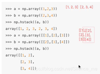
numpy.vstack(tup)
numpy.concatenate((a1, a2 , ...), axis=0)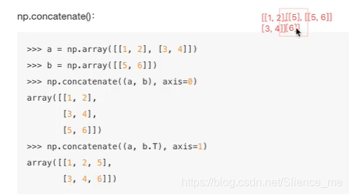

python

a = stock_change[:2, 0:4]
b = stock_change[4:6, 0:4]

a
array([[1.1, -0.45576704, 0.29667843, 0.16606916],
       [0.36775845, 0.24078108, 0.122042, 1.1]])

a.shape  # (2, 4)

a.reshape((-1, 2))
array([[1.1, -0.45576704],
       [0.29667843, 0.16606916],
       [0.36775845, 0.24078108],
       [0.122042, 1.1]])

b
array([[-0.9822216, -1.09482936, -0.81834523, 1.1],
       [0.41739964, -0.26826893, -0.70003442, -0.58593912]])

np.hstack((a, b))
array([[1.1, -0.45576704, 0.29667843, 0.16606916, -0.9822216,
        -1.09482936, -0.81834523, 1.1],
       [0.36775845, 0.24078108, 0.122042, 1.1, 0.41739964,
        -0.26826893, -0.70003442, -0.58593912]])

np.concatenate((a, b), axis=1)
array([[1.1, -0.45576704, 0.29667843, 0.16606916, -0.9822216,
        -1.09482936, -0.81834523, 1.1],
       [0.36775845, 0.24078108, 0.122042, 1.1, 0.41739964,
        -0.26826893, -0.70003442, -0.58593912]])

np.vstack((a, b))
array([[1.1, -0.45576704, 0.29667843, 0.16606916],
       [0.36775845, 0.24078108, 0.122042, 1.1],
       [-0.9822216, -1.09482936, -0.81834523, 1.1],
       [0.41739964, -0.26826893, -0.70003442, -0.58593912]])

np.concatenate((a, b), axis=0)
array([[1.1, -0.45576704, 0.29667843, 0.16606916],
       [0.36775845, 0.24078108, 0.122042, 1.1],
       [-0.9822216, -1.09482936, -0.81834523, 1.1],
       [0.41739964, -0.26826893, -0.70003442, -0.58593912]])

6.2 分割

7. IO操作与数据处理

7.1 Numpy读取

python

data = np.genfromtxt("test.csv", delimiter=",")

array([[nan, nan, nan, nan],
       [1., 123., 1.4, 23.],
       [2., 110., nan, 18.],

python

def fill_nan_by_column_mean(t):
  for i in range(t.shape[1]):
    # 计算nan的个数
    nan_num = np.count_nonzero(t[:, i][t[:, i] != t[:, i]])
    if nan_num > 0:
      now_col = t[:, i]
      # 求和
      now_col_not_nan = now_col[np.isnan(now_col) == False].sum()
      # 和/个数
      now_col_mean = now_col_not_nan / (t.shape[0] - nan_num)
      # 赋值给now_col
      now_col[np.isnan(now_col)] = now_col_mean
      # 赋值给t，即更新t的当前列
      t[:, i] = now_col
  return t

7.2 如何处理缺失值

两种思路：

直接删除含有缺失值的样本
替换/插补
- 按列求平均，用平均值进行填补

发布时间:

2021-08-16

Python-Numpy简单了解 ​

1. Numpy优势 ​

1.1 Numpy介绍 - 数值计算库 ​

1.2 ndarray介绍 ​

1.3 ndarray与Python原生list运算效率对比 ​

1.4 ndarray的优势 ​

2. 认识N维数组-ndarray属性 ​

2.1 ndarray的属性 ​

2.2 ndarray的形状 ​

2.3 ndarray的类型 ​

3. 基本操作 ​

3.1 生成数组的方法 ​

3.1.1 生成0和1 ​

3.1.2 从现有数组中生成 ​

3.1.3 生成固定范围的数组 ​

3.1.4 生成随机数组 ​

3.2 数组的索引、切片 ​

3.3 形状修改 ​

3.4 类型修改 ​

3.5 数组的去重 ​

4. ndarray运算 ​

4.1 逻辑运算 ​

4.2 统计运算 ​

5. 数组间运算 ​

5.1 场景 ​

5.2 数组与数的运算 ​

5.3 数组与数组的运算 ​

5.4 广播机制 ​

5.5 矩阵运算 ​

6. 合并、分割 ​

6.1 合并 ​

6.2 分割 ​

7. IO操作与数据处理 ​

7.1 Numpy读取 ​

7.2 如何处理缺失值 ​

Python-Numpy简单了解

1. Numpy优势

1.1 Numpy介绍 - 数值计算库

1.2 ndarray介绍

1.3 ndarray与Python原生list运算效率对比

1.4 ndarray的优势

2. 认识N维数组-ndarray属性

2.1 ndarray的属性

2.2 ndarray的形状

2.3 ndarray的类型

3. 基本操作

3.1 生成数组的方法

3.1.1 生成0和1

3.1.2 从现有数组中生成

3.1.3 生成固定范围的数组

3.1.4 生成随机数组

3.2 数组的索引、切片

3.3 形状修改

3.4 类型修改

3.5 数组的去重

4. ndarray运算

4.1 逻辑运算

4.2 统计运算

5. 数组间运算

5.1 场景

5.2 数组与数的运算

5.3 数组与数组的运算

5.4 广播机制

5.5 矩阵运算

6. 合并、分割

6.1 合并

6.2 分割

7. IO操作与数据处理

7.1 Numpy读取

7.2 如何处理缺失值